Tutorial
Skeleton Module
As mentioned on the Avizo Scripts page, the FIBbootstrap.skeleton
module expects a series of *.mv3d skeleton files and *.csv statistic
files that were output by these methods.
Once these are obtained, it is relatively simple to obtain confidence intervals
using the bootstrap_skel_stats() method.
A bit of example code that would work is shown below. In this example,
you give the path to the .mv3d files, and then specify a couple wildcard
patterns that match the files you have (these will obviously be different in
your case). Then, we loop through the patterns, calling
bootstrap_skel_stats() on each pattern.
For each iteration, it finds the .csv files automatically, and saves the
data and error output to two .csv files in the current directory.
The volume parameter enable the calculation of node and edge density,
in addition to just the raw node and edge counts.
>>> import os
>>> import FIBbootstrap.skeleton as fb_skel

>>> directory =  "/path/to/mv3d/files"

>>> mv3d_pattern1 = "1subvolSkel.*.mv3d"
>>> mv3d_pattern2 = "2subvolSkel.*.mv3d"
>>> mv3d_pattern3 = "3subvolSkel.*.mv3d"

>>> for pat in [mv3d_pattern1, mv3d_pattern2, mv3d_pattern3]:
...     data, err = fb_skel.bootstrap_skel_stats(os.path.join(directory, pat),
...                                              save_output=True, volume=4**3)
Here is an example of the data output from some of my data. It contains the skeleton quantification for each subvolume (real data is 500 subvolumes, but only 5 are shown here):
| E | E/V | N | N/V | mean_k | perc_deg | topo_length | |
|---|---|---|---|---|---|---|---|
| 0 | 461.0 | 7.2 | 310.0 | 4.84 | 2.97 | 0.9974 | 946.5 |
| 1 | 581.0 | 9.08 | 386.0 | 6.03 | 3.01 | 1.0 | 548.5 |
| 2 | 455.0 | 7.11 | 309.0 | 4.83 | 2.94 | 1.0 | 989.6 |
| 3 | 416.0 | 6.5 | 277.0 | 4.33 | 3.0 | 1.0 | 926.3 |
| 4 | 379.0 | 5.92 | 268.0 | 4.19 | 2.83 | 1.0 | 1011.2 |
The error output contains the same quantifications, but as various descriptive statistics. The first two are the most important, and represent the asymmetric confidence interval errors, as calculated using the bootstrap method. The remaining three rows represent the mean, standard deviation, and standard error of the mean for the subvolumes that were analyzed. Comparing the mean of the subvolumes to the overall value that was obtained can be a good way of determining whether the small volumes are representative of the larger overall one. Here is an example of the error output:
| E | E/V | N | N/V | mean_k | perc_deg | topo_length | |
|---|---|---|---|---|---|---|---|
| Neg. CI | 14.6 | 0.23 | 9.5 | 0.15 | 0.01 | 0.0001 | 34.0 |
| Pos. CI | 13.9 | 0.22 | 9.0 | 0.14 | 0.01 | 0.0001 | 36.2 |
| Mean | 459.5 | 7.18 | 312.9 | 4.89 | 2.93 | 0.9998 | 889.0 |
| Std. Dev. | 73.1 | 1.14 | 47.3 | 0.74 | 0.05 | 0.0005 | 178.8 |
| SEM | 7.3 | 0.11 | 4.7 | 0.07 | 0.0 | 0.0 | 17.9 |
Surfaces Module
The FIBbootstrap.surface module expects a series of *.csv
surface statistic files that were output by the Subvolume surface
Avizo script. Running the analysis is fairly easy, but this module is specifically
designed for my samples and data, so it will need to be tailored to your needs.
In fact, it would probably be easiest to copy the
process_surface_stats_lsm_ysz() and modify it
to your data.
The method primarily is just a wrapper for some pandas manipulations
that calculate various properties, such as phase volume normalized surface area,
average particle size (using the BET formula), phase volume fraction,
and solid phase fraction. To use it, some code like the following will work,
assuming you have a directory containing a number of surface statistics
*.csv files output by the Avizo script. The process_surface_stats_lsm_ysz()
method will parse these files and calculate the same sort of error statistics
as the Skeleton Module.
The following code will look for two sets of .csv files matching the
patterns pat1 and pat2, looping through them all, and create an output
.csv file for each pattern, named according to the names given
in the dict_ parameter.
>>> from FIBbootstrap import surface as fb_surf

>>> pat1 = "1subvolSurf*.csv"
>>> pat2 = "2subvolSurf*.csv"

>>> dict_ = {'name1': pat1,
...          'name2': pat2}

>>> for sample, pattern in dict_.items():
...      fb_surf.process_surface_stats_lsm_ysz(pattern,
...                                            save_output=True,
...                                            output_fname=sample + '_surface_bootstrap_errors.csv')
Running this code will produce a .csv file with contents like shown below.
In this example, the YSZ and Pore results have been excluded for clarity, but
results for those materials would be calculated as well.
| LSM_volNormSA | LSM_BET_d | LSM_volFrac | LSM_solVolFrac | |
|---|---|---|---|---|
| Neg. CI | 0.0002 | 23.2 | 0.008 | 0.01 |
| Pos. CI | 0.0002 | 27.2 | 0.009 | 0.01 |
| Mean | 0.0073 | 867.2 | 0.288 | 0.49 |
| Std. Dev. | 0.0015 | 220.9 | 0.077 | 0.1 |
| SEM | 0.0001 | 12.8 | 0.004 | 0.01 |
Tortuosity Module
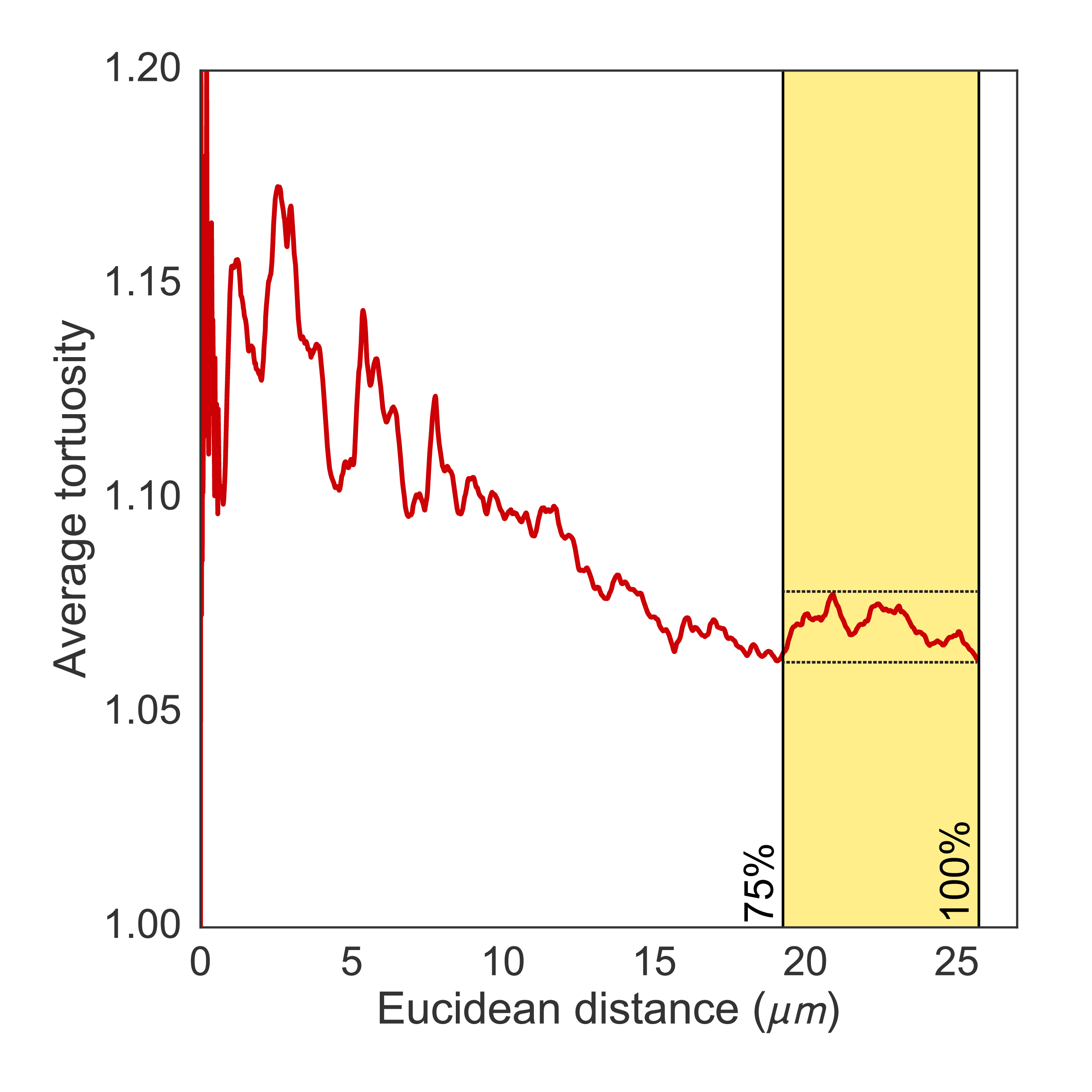
The tortuosity of a phase cannot be very effectively calculated on a subvolume of the sample, since its value is dependent on a limit (see the paper referenced in Introduction), and the reduced volume will artificially inflate the value of tortuosity found. As such, the estimated error is measured by looking at the standard deviation of the final ~25% of the tortuosity profile, as shown below:
These profiles are created by the fibtortuosity.tortuosity_profile()
method, and the bootstrap_tort_stats() method
of the Bootstrap module will easily calculate the error values from these profiles.
This method will load each profile found in a directory (specified with the
pattern parameter, and calculate descriptive statistics based off the last
fraction of each profile (specified with the threshold parameter). Multiple
samples in different directories can be analyzed by putting more patterns
into the dictionary, as shown below:
>>> import FIBbootstrap.tortuosity as fb_tort

>>> pat = "*profile.csv"
>>> dict_ = {'sample1': pat}

>>> for sample, pattern in dict_.items():
...      fb_tort.bootstrap_tort_stats(pattern,
...                                   save_output=True,
...                                   threshold=0.75,
...                                   data_output_fname=sample + '_bootstrap_data.csv',
...                                   err_output_fname=sample + '_bootstrap_errors.csv')
The result of this code will be two .csv files in the current directory.
The first is the data file, which will contain all of the tortuosity profiles
found, with one column per profile loaded (and without the euclidean distance data).
Here is an example of the first few rows of the data file for an example
from my research:
| Pore y | YSZ x | Pore x | LSM y | Pore z | LSM x | YSZ z | LSM z | YSZ y | |
|---|---|---|---|---|---|---|---|---|---|
| 0 | 1.02 | 1.064 | 1.014 | 1.132 | 1.04 | 1.676 | 1.128 | 1.679 | 1.064 |
| 1 | 1.02 | 1.064 | 1.014 | 1.132 | 1.04 | 1.679 | 1.127 | 1.673 | 1.064 |
| 2 | 1.02 | 1.064 | 1.014 | 1.132 | 1.04 | 1.682 | 1.127 | 1.666 | 1.064 |
| 3 | 1.02 | 1.065 | 1.014 | 1.132 | 1.041 | 1.685 | 1.127 | 1.66 | 1.064 |
| 4 | 1.021 | 1.065 | 1.014 | 1.132 | 1.041 | 1.688 | 1.128 | 1.653 | 1.065 |
The other file output will be the error .csv file. This will have the
same format as the other error reports output by the modules in this package,
and for each profile found, will report the confidence intervals, the mean,
standard deviation, etc. In our opinion, the standard deviation is the best
value to use for the error.
| Pore y | YSZ x | Pore x | LSM y | Pore z | LSM x | YSZ z | LSM z | YSZ y | |
|---|---|---|---|---|---|---|---|---|---|
| Neg. CI | 0.0 | 0.0 | 0.0 | 0.001 | 0.0 | 0.026 | 0.001 | 0.013 | 0.0 |
| Pos. CI | 0.0 | 0.0 | 0.0 | 0.001 | 0.0 | 0.028 | 0.001 | 0.014 | 0.0 |
| Mean | 1.02 | 1.07 | 1.018 | 1.143 | 1.039 | 1.4 | 1.12 | 1.562 | 1.063 |
| Std. Dev. | 0.001 | 0.003 | 0.002 | 0.009 | 0.001 | 0.169 | 0.006 | 0.055 | 0.003 |
| SEM | 0.0 | 0.0 | 0.0 | 0.001 | 0.0 | 0.014 | 0.001 | 0.007 | 0.0 |
TPB Module
Calculation
Because the definition of TPB activity depends on the intersection of phase
components (see the paper referenced in Introduction), it does not make
sense to calculate discrete TPB networks on smaller subvolumes of the original
LabelField, since the activity will be artificially inflated due to the reduced
volume. Rather, the FIBbootstrap.tpb module will instead take a total
TPB network, and subsample it internally, calculating the fraction of active vs.
inactive in each subvolume.
The expected input is a dictionary with three input files for the active,
inactive, and unknown TPB networks of a sample. The networks are obtained
by using the tpbLen.py script. The resulting output of this script
is an Avizo SpatialGraph file (.am), which should then be converted into .mv3d format
using Avizo (the script could certainly be modified to work on different formats,
but this is what was convenient for our research).
Code such as the following will calculate the total active, inactive, and unknown
TPB length, as well as the TPB density, for n_volumes number of subvolumes.
The box size can be provided as well:
>>> import FIBbootstrap.tpb as fb_tpb

>>> input_dict = {'A': 'smoothActive.savg.mv3d',
...               'I': 'smoothInactive.savg.mv3d',
...               'U': 'smoothUnknown.savg.mv3d'}

>>> data_out, \
... error_out = fb_tpb.bootstrap_tpb_stats(input_dict,
...                                        n_volumes=500,
...                                        box_size=4000,
...                                        save_output=True,
...                                        data_output_fname='data_N500_s4000.csv',
...                                        err_output_fname='errors_N500_s4000.csv',
...                                        output_avg=False)
The bootstrap_tpb_stats() method will return two
pandas.DataFrame objects. The first (data_out) holds
the results for each random subvolume calculated. The second (`error_out)
holds the error calculations, like the other modules in this package.
Using the save_output parameter will enable saving of .csv files for
each of these DataFrames.
The first few rows of an example TPB data output is as follows:
| A_TPBdens | A_totL | I_TPBdens | I_totL | U_TPBdens | U_totL | |
|---|---|---|---|---|---|---|
| 0 | 3.09 | 197.81 | 0.84 | 53.91 | 1.07 | 68.79 |
| 1 | 1.59 | 101.56 | 0.64 | 41.15 | 0.29 | 18.36 |
| 2 | 2.64 | 169.11 | 0.98 | 62.68 | 0.45 | 28.6 |
| 3 | 2.57 | 164.53 | 1.11 | 70.75 | 0.14 | 8.65 |
| 4 | 2.56 | 164.07 | 0.3 | 19.25 | 0.6 | 38.13 |
The error output appears as such:
| A_TPBdens | A_totL | I_TPBdens | I_totL | U_TPBdens | U_totL | |
|---|---|---|---|---|---|---|
| Neg. CI | 0.06 | 3.88 | 0.04 | 2.75 | 0.03 | 2.23 |
| Pos. CI | 0.06 | 3.9 | 0.05 | 2.91 | 0.04 | 2.44 |
| Mean | 2.47 | 158.06 | 1.22 | 78.14 | 0.58 | 37.14 |
| Std. Dev. | 0.69 | 44.17 | 0.5 | 32.26 | 0.41 | 26.55 |
| SEM | 0.03 | 1.98 | 0.02 | 1.44 | 0.02 | 1.19 |
Visualization
If the mayavi.mlab module is installed, it can be used to
visualize a little animation showing the TPB and how it is being subsampled.
The function to do this is animate_cropped_data.
If everything is installed correctly, it should create two windows with interactive visualizations of the TPB network. One will show the entire network, and another will show the subvolumes (and the TPB networks inside of them) that are created by the subsampling code in this module. The visualization helps provide some affirmation that the method is sampling the volume randomly as expected.
To create thee visualization, the following code can be used (assuming you have TPB networks with the filenames indicated below):
>>> import FIBbootstrap.tpb as fb_tpb

>>> size = 4000

>>> data_a, num_lines_a, num_points_a = fb_tpb.read_mv3d('smoothActive.savg.mv3d')
>>> data_i, num_lines_i, num_points_i = fb_tpb.read_mv3d('smoothInactive.savg.mv3d')
>>> data_u, num_lines_u, num_points_u = fb_tpb.read_mv3d('smoothUnknown.savg.mv3d')

>>> fb_tpb.animate_cropped_data(data_a, data_i, data_u,
...                             size, 2)
This should result in an animation such as the following, showing the full TPB network in one window (colored by active, inactive, or unknown), and the reduced network from the random subvolume in the other:
Utilities Module
The only method in the utils module is
calculate_errors(). It shouldn’t have to
be used directly, but is used by each of the modules in this package.
It is very generic, and is the heart of the code that calculates the
confidence intervals and descriptive statistics for a pandas.DataFrame.
Given any DataFrame df, the method can be used with a single call,
where n_bootstrap is the number of bootstrap iterations to use:
>>> error_df = calculate_errors(df, n_bootstrap)
This will produce a DataFrame containing the same information as the error
.csv files as described above.